Life can only be understood going backwards, but it must be lived going forwards - Kierkegaard.
Dynamic Programming is a mathematical technique that is used in several fields of research including economics, finance, engineering. It deals with making decisions over different stages of the problem in order to minimize (or maximize) a corresponding cost function (or reward). The outcome of a decision at a given stage can be fully predicted (deterministic) or can only be partially predicted (with randomness involved). One key aspect of such problems is the trade off in optimizing the cost incurred at the current stage and the cost to be incurred at a future stage.
Dynamic Programming is very helpful in many contexts by providing an exact solution, however, when the problem size increases, it requires enormous amount of storage and computational time (often referred to as the curse of dimensionality) which makes it infeasible to apply to practical situations. Often in such situations, one may not desire an exact solution, but an approximately optimal (or suboptimal) solution. Then there must be a better class of techniques that can capture this trade off between feasibility and sub optimality. These techniques are collectively referred to as Approximate Dynamic Programming or Reinforcement Learning (in the field of AI) or Neuro Dynamic Programming (in the field of automatic control), all of which essentially mean the same.
In this blog post, we shall look at a specific technique called Rollout Algorithm that is quite extensively used (with surprisingly good results). In fact, Mastering the game of Go, DeepMind uses a variant of Rollout called Monte Carlo Tree Search. We shall first formulate a DP problem, state the DP algorithm and illustrate with an example the infeasibility of DP. Using the same example, we shall study how Rollout offers an effective solution that optimizes the trade-off between accuracy and computation. This post is entirely based on my reading of the book Approximate Dynamic Programming.
DP formulation
In this post, we shall focus only on finite horizon problems (problems involving a finite number of stages or time steps at which a decision is taken). We denote the state of the system at time $k$ as $x{_k}$ (belongs to a space $S{_k}$ ), and the decision (or control) taken as $u{_k}$ (belongs to a space $U{_k} (x{_k}) $ ), and a random variable $w{_k}$ (which is independent of other $w{_i}$) that affects the system. The system has the form
$$x_{k+1} = f_{k}(x_{k}, u_{k}, w_{k})$$
where $k$ takes a value between $0$ and $N$ (finite horizon). At each stage, there is a cost incurred $g{_k}(x{_k}, u{_k}, w{_k})$ which accumulates over time. The total cost incurred is then
$$ g_{N}(x_{N}) + \sum_{k=0}^{N-1}g_{k}(x_{k}, u_{k}, w_{k})$$
where $g {_N}(x{_N})$ is a terminal cost incurred at the final stage (it only depends on the state, and no action is to be taken). The objective of the problem is to find an optimal policy
$$\pi:= {\mu_{0},..,\mu_{k},.. \mu_{N-1}}$$
(where $\mu_{k} = u_{k}(x_{k})$) that minimizes the expected cost (we take an expectation due to the random variable $w_{k}$). Given an initial state $x_{0}$, the expected cost of following a policy $\pi$ starting from $x_0$ is denoted as
$$ J_{\pi}(x_{0}) = \mathbb{E}\big[g_{N}(x_{N}) + \sum_{k=0}^{N-1}g_{k}(x_{k}, u_{k}, w_{k})]$$
An optimal policy $\pi^{*}$ is the one that minimizes this expected cost; i.e,
$$ J_{\pi^{*}}(x_{0}) = \min_{\pi \in \Pi} J_{\pi}(x_{0})$$
where $\Pi$ is the space of admissible policies.
Bellman’s principle of optimality
Let $\pi^{*}={\mu_{0}^{*},..,\mu_{k}^{*},.. \mu_{N-1}^{*}}$ be an optimal policy of the problem stated above, and assume that when using $\pi^{*}$, a given state $x_{i}$ occurs at time $i$ with positive probability. Consider the subproblem, whereby we are at $x_{i}$ at time $i$ and wish to minimze the “cost-to-go” from time $i$ to time $N$
$$ \mathbb{E}\bigg[g_{N}(x_{N}) + \sum_{k=i}^{N-1}g_{k}(x_{k}, u_{k}, w_{k})\bigg]$$
Then the truncated policy ${\mu_{i}^{*},\mu_{i+1}^{*},.. \mu_{N-1}^{*}}$ is optimal for this subproblem.
Intuitively, let us look at the following problem where we start from A and we need to reach the destination E, and the edge weights are the costs incurred for traversing that edge. The path that minimizes the cost is A-B-D-E. Equivalently, the decision (corresponds to choosing the next node) taken at each time step are B at k=0, D at k=1 and E at k=2. If the policy determined by the path A-B-D-E is optimal, then the truncated path B-D-E is also optimal. If it were not, then we can further reduce the cost by choosing the optimal path which contradicts the fact that A-B-D-E is the path with the minimum cost.

DP Illustration
DP Algorithm
The DP algorithm proceeds as follows. We start from the last step of decision making ($N-1$) and proceed backwards performing the minimization
$$ J_{N}(x_{N}) = g_{N}(x_{N}) $$
$$ J_{k}(x_{k}) =\min_{u_{k} \in U_{k}(x_{k})}\mathbb{E}_{w_{k}}\bigg[g_{k}(x_{k}, u_{k}, w_{k}) + J_{k+1}(f_{k}(x_{k}, u_{k}, w_{k}))\bigg],$$ $$ k = 0,1,..,N-1$$
where the expectation is taken with respect to the probability distribution of $w_{k}$ which is assumed to depend on $x_{k}, u_{k}$. Furthermore, if $\mu^{*}_{k}=u_{k}^{*}(x_{k})$ minimizes the above equation, then the policy $\pi^{*}={\mu_{0}{*},…,\mu_{k}{*},…,\mu_{N-1}{*}}$ is optimal.
Example
Let us look at an example application of the above described DP algorithm. Consider a perfect binary tree of height N (i.e. each level k of the binary tree has $2^{k}$ nodes). The nodes are of two types, green and red. It is know before hand that each node can be red with probability $p$ and green with probability $1-p$. We shall call an arc as the line joining a node with one of it’s children. An arc is free if both the nodes are green, and is blocked if either of them is red. One can only traverse along free arcs, and the objective is to find if a free path (a sequence of free arcs) exists from the root to the leaves.

Free path
One way to find an exact solution to the above problem is to use DP to start from the leaves (level N), and traverse backwards to check if a free path exists. In the $k^{th}$ step of the DP, the algorithm finds if a path exists from each node (at height $N-k$) to the leaves using the results from step $k-1$. The amount of computation at the $k^{th}$ step is $\mathcal{O}(2^{N-k})$ and there are $N$ steps in the algorithm. The overall runtime is of the order $\mathcal{O}(N2^{N})$. We can see from the plot that the run time increases exponentially with the height of the tree.
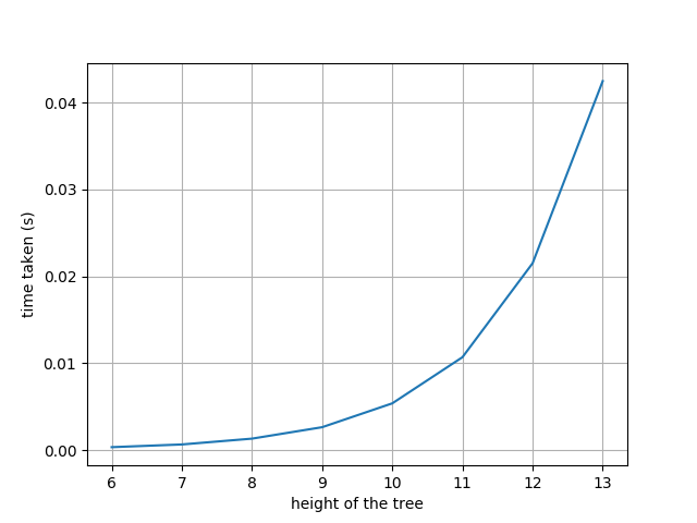
Run time plot
In problems where finding an exact solution is not critical and finding an approximately correct solution (that works most of the time) is sufficient, faster heuristics can be employed to achieve a tradeoff between accuracy and computation. Let us use one such heuristic here that reduces the computation time drastically while offering a suboptimal solution.
Consider a greedy algorithm which starts at the root node. If both the arcs from the root node are blocked, then the algorithm returns False (no path exists). If one of the arcs is free, it traverses down that arc to the child node and repeats the same with this node. If both the arcs are free, then it uses a fixed rule to choose which arc to traverse (say it chooses always the right arc). The runtime of this algorithm is $\mathcal{O}(N)$ which is extremely fast as compared to $\mathcal{O}(N2^{N})$. However, this algorithm always doesn’t output the correct solution. For example, in the above figure, this algorithm outputs False despite the existence of a free path (bold lines).
One-step lookahead
One effective way to reduce the computation is to use an approximate cost-to-go function. In the DP algorithm, to obtain the control at $k$ we perform the minimization over all possible exact $J_{k+1}(f_{k}(x_{k}, u_{k}, w_{k}))$. Instead if we are able to approximate the cost to go of stage $k+1$ as $\tilde{J}_{k+1}(f_{k}(x_{k}, u_{k}, w_{k}))$, we can avoid the computation required to minimize over all the next stages. This is called a one step lookahead policy, where at stage $k$ we perform the following minimization
$$\bar{\mu}_{k}(x_{k}) = \arg \min_{u_{k} \in U_{k}(x_{k})}\mathbb{E}_{w_{k}}\bigg[g_{k}(x_{k}, u_{k}, w_{k}) + \tilde{J}_{k+1}(f_{k}(x_{k}, u_{k}, w_{k}))\bigg],$$ $$k = 0,1,..,N-1$$
and the one step lookahead policy is denoted as $\bar{\pi}=\{ \bar{\mu}_{0},…,\bar{\mu}_{N-1} \}$
Similarly, in a two step lookahead policy, we use the same minimization as above, but instead of directly using $\tilde{J}_{k+1}(f_{k}(x_{k}, u_{k}, w_{k}))$, we obtain it as a minimization of a one step lookahead approximation.
$$ \tilde{J}_{k+1}(x_{k+1}) =\min_{u_{k+1} \in U_{k+1}(x_{k+1})}\mathbb{E}_{w_{k+1}}\bigg[g_{k+1}(x_{k+1}, u_{k+1}, w_{k+1}) + \\
J_{k+2}(f_{k+1}(x_{k+1}, u_{k+1}, w_{k+1}))\bigg], k = 0,1,..,N-2$$
where $\tilde{J}_{k+2}$ is an approximation of the cost-to-go of $J_{k+2}$. Intuitively, it can be described as solving a two level DP at every stage of the problem. If the cost-to-go function can be approximated fairly accurately, then this algorithm can provide an approximate solution in a much better run time as compared to solving the complete DP. Now arises the most important question, how do we approximate the cost-to-go function? Infact, most of the recent research in this field is dedicated towards finding computationally feasible techniques that provide approximately accurate representations for the cost functions. Following are some types of approximation techniques,
- Problem approximation: Lookahead techniques described above approximate the problem to a limited number of steps at every stage of the algorithm
- Parametric cost approximation: The cost-to-go functions are approximated from a parametric class of functions (for example, neural networks)
- On-line approximation: A suboptimal policy is used on-line to approximate the cost-go-function. In this article, we shall look at Rollout algorithm that belongs to this approach
- Simulation-based approximation: In the presence of a simulator that can accurately determine the state transitions of the problem, Monte Carlo simulations are used to approximate the cost functions.
Rollout
The Rollout algorithm is similar to a one step lookahead algorithm in the sense that we find the control that minimizes the expression $$\bar{\mu}_{k}(x_{k}) = \arg \min_{u_{k} \in U_{k}(x_{k})}\mathbb{E}_{w_{k}}\bigg[g_{k}(x_{k}, u_{k}, w_{k}) + \tilde{J}_{k+1}(f_{k}(x_{k}, u_{k}, w_{k}))\bigg],$$ $$k = 0,1,..,N-1$$
where $\tilde{J}_{k+1}$ is the true cost-to-go of $J_{k+1}$ with respect to a suboptimal base policy $\pi$. The policy thus obtained $\bar{\pi}=\{ \bar{\mu}_{0},…,\bar{\mu}_{N-1} \}$ is called the rollout policy. Since in the minimization, at each stage we always choose the control that minimizes the true cost-to-go of the suboptimal policy, the cost-to-go approximation is always less than or equal to the cost-to-go of the base policy. The rollout algorithm thus yields a policy better than the base policy. This technique is called as policy improvement.
Let us now apply this rollout algorithm to the example we discussed above. The rollout algorithm proceeds as follows.
- If at a node, at least one of the two children is red, it proceeds exactly like the greedy algorithm.
- If at a node, both the children are green, rollout algorithm looks one step ahead, i.e. runs greedy policy on the children of the current node. If exactly one of these return True, the algorithm traverses that corresponding arc. If both of these return True, then the algorithm chooses one according to a fixed rule (choose the right child), and if both of them return False, then the algorithm returns False.
This seemingly very simple trick can lead to large performance gains while minimizing the computation required. If we look at the results below, we can observe that using rollout we can considerable improve on the accuracy of finding a free path, while keeping the amount of computation required close to that of the greedy policy. The implementation can be found here.

Accuracy plot
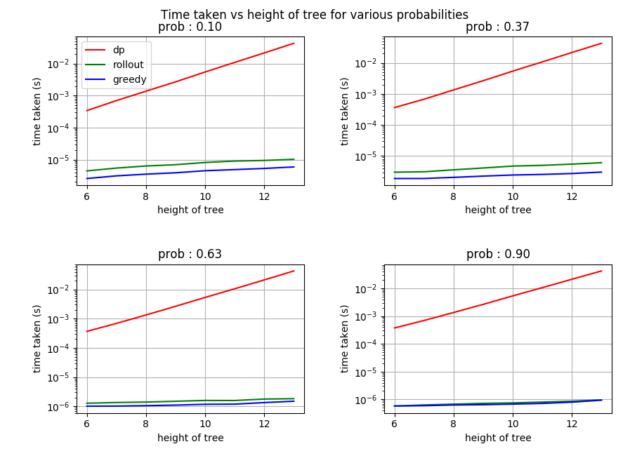
Runtime plot
Conclusion
In this post, we discussed the basic DP problem, formulation, algorithm and illustrated with an example the infeasibility of using the DP algorithm. In problems where a suboptimal solution is sufficient, we discussed the rollout algorithm that improves upon the performance of a greedy base policy while requiring minimal computation.
References
- Bertsekas, D. P. (1995). Dynamic programming and optimal control (Vol. 1, No. 2). Belmont, MA: Athena scientific.